Evaluation¶

Slideflow includes several tools for evaluating trained models. In the next sections, we’ll review how to evaluate a model on a held-out test set, generate predictions without ground-truth labels, and visualize predictions with heatmaps.

Evaluating a test set¶

The slideflow.Project.evaluate() provides an easy interface for evaluating model performance on a held-out test set. Locate the saved model to evaluate (which will be in the project models/ folder). As with training, the dataset to evaluate can be specified using either the filters or dataset arguments. If neither is provided, all slides in the project will be evaluated.

# Method 1: specifying filters
P.evaluate(
  model="/path/to/trained_model_epoch1",
  outcomes="tumor_type",
  filters={"dataset": ["test"]}
)

# Method 2: specify a dataset
dataset = P.dataset(tile_px=299, tile_um='10x')
test_dataset = dataset.filter({"dataset": ["test"]})
P.evaluate(
  model="/path/to/trained_model_epoch1",
  outcomes="tumor_type",
  dataset=test_dataset
)

Results are returned from the Project.evaluate() function as a dictionary and saved in the project evaluation directory. Tile-, slide-, and patient- level predictions are also saved in the corresponding project evaluation folder, eval/.

Generating predictions¶

For a dataset¶

slideflow.Project.predict() provides an interface for generating model predictions on an entire dataset. As above, locate the saved model from which to generate predictions, and specify the dataset with either filters or dataset arguments.

dfs = P.predict(
  model="/path/to/trained_model_epoch1",
  filters={"dataset": ["test"]}
)
print(dfs['patient'])

                        patient  ...  cohort-y_pred1
  TCGA-05-4244-01Z-00-DX1...  ...        0.032608
  TCGA-05-4245-01Z-00-DX1...  ...        0.216634
  TCGA-05-4249-01Z-00-DX1...  ...        0.000858
  TCGA-05-4250-01Z-00-DX1...  ...        0.015915
  TCGA-05-4382-01Z-00-DX1...  ...        0.020700
..                          ...  ...             ...
TCGA-O2-A52S-01Z-00-DX1...  ...        0.983500
TCGA-O2-A52V-01Z-00-DX1...  ...        0.773328
TCGA-O2-A52W-01Z-00-DX1...  ...        0.858558
TCGA-S2-AA1A-01Z-00-DX1...  ...        0.000212
TCGA-XC-AA0X-01Z-00-DX1...  ...        0.632612

Results are returned as a dictionary of pandas DataFrames (with the keys 'tile', 'slide', and 'patient' for each level of prediction) and saved in the project evaluation directory, eval/.

For a single slide¶

You can also generate predictions for a single slide with either slideflow.slide.predict() or slideflow.WSI.predict().

import slideflow as sf

slide = '/path/to/slide.svs'
model = '/path/to/model_epoch1'
sf.slide.predict(slide, model)

array([0.84378019, 0.15622007])

The returned array has the shape (num_classes,), indicating the whole-slide prediction for each outcome category. If the model was trained with uncertainty quantification, this function will return two arrays; the first with predictions, the second with estimated uncertainty.

Heatmaps¶

For a dataset¶

Predictive heatmaps can be created for an entire dataset using slideflow.Project.generate_heatmaps(). Heatmaps will be saved and exported in the project directory. See the linked API documentation for arguments and customization.

P.generate_heatmaps(model="/path/to/trained_model_epoch1")

For a single slide¶

slideflow.Heatmap provides more granular control for calculating and displaying a heatmap for a given slide. The required arguments are:

slide: Either a path to a slide, or a slideflow.WSI object.
model: Path to a saved Slideflow model.

Additional keyword arguments can be used to customize and optimize the heatmap. In this example, we’ll increase the batch size to 64 and allow multiprocessing by setting num_processes equal to our CPU core count, 16.

heatmap = sf.Heatmap(
  slide='/path/to/slide.svs',
  model='/path/to/model'
  batch_size=64,
  num_processes=16
)

If slide is a slideflow.WSI, the heatmap will be calculated only within non-masked areas and ROIs, if applicable.

from slideflow.slide import qc

# Prepare the slide
wsi = sf.WSI('slide.svs', tile_px=299, tile_um=302, rois='/path')
wsi.qc([qc.Otsu(), qc.Gaussian()])

# Generate a heatmap
heatmap = sf.Heatmap(
  slide=wsi,
  model='/path/to/model'
  batch_size=64,
  num_processes=16
)

If slide is a path to a slide, Regions of Interest can be provided through the optional roi_dir or rois arguments.

Once generated, heatmaps can be rendered and displayed (ie. in a Jupyter notebook) with slideflow.Heatmap.plot().

heatmap.plot(class_idx=0, cmap='inferno')

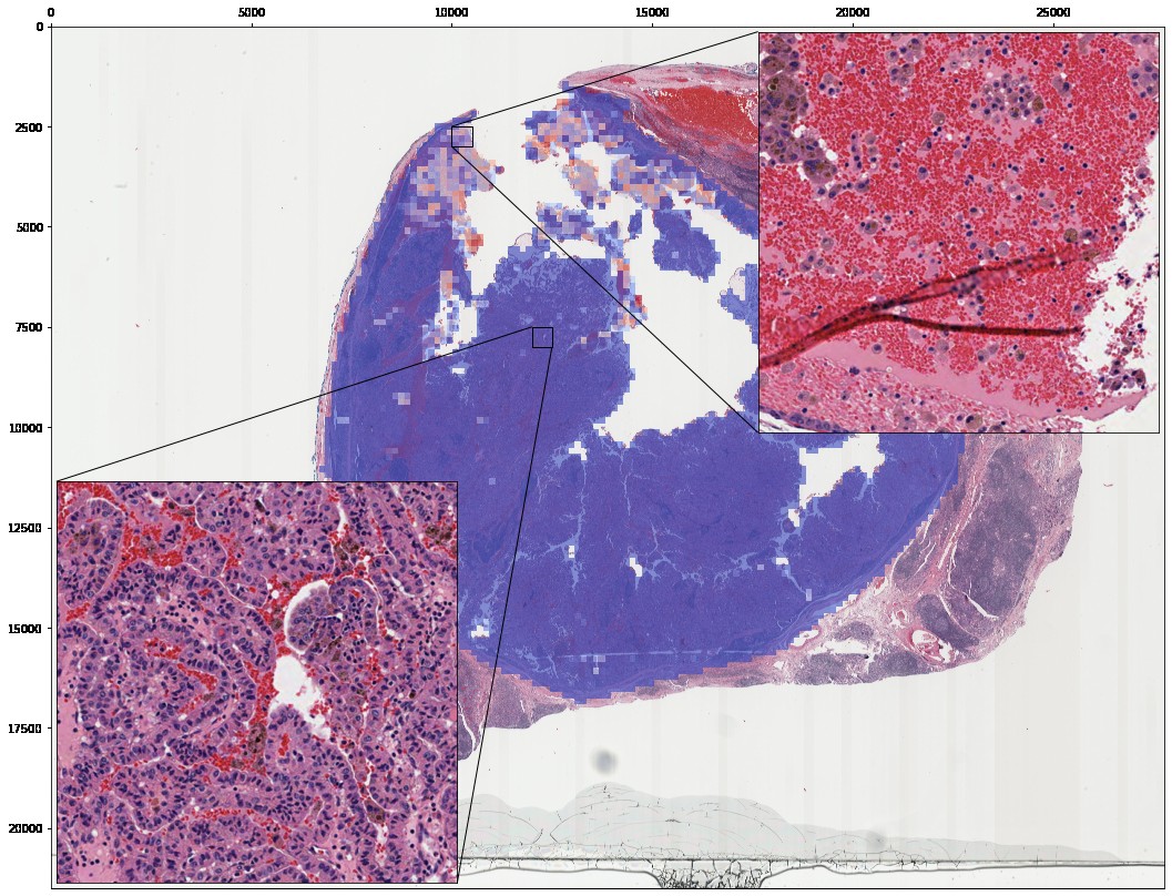
Insets showing zoomed-in portions of the heatmap can be added with slideflow.Heatmap.add_inset():

heatmap.add_inset(zoom=20, x=(10000, 10500), y=(2500, 3000), loc=1, axes=False)
heatmap.add_inset(zoom=20, x=(12000, 12500), y=(7500, 8000), loc=3, axes=False)
heatmap.plot(class_idx=0, mpp=1)

Save rendered heatmaps for each outcome category with slideflow.Heatmap.save(). The spatial map of predictions, as calculated across the input slide, can be accessed through Heatmap.predictions. You can save the numpy array with calculated predictions (and uncertainty, if applicable) as an *.npz file using slideflow.Heatmap.save_npz().