Saliency Maps¶

Slideflow provides an API for calculating gradient-based pixel attribution (saliency maps), as implemented by PAIR. Saliency maps can be calculated manually (as described below), or interactively in Slideflow Studio.

slideflow.grad.SaliencyMap provides an interface for preparing a saliency map generator from a loaded model (Tensorflow or PyTorch) and calculating maps from preprocessed images. Supported methods include:

Vanilla gradients
Integrated gradients
Guided integrated gradients
Blur integrated gradients
XRAI
Grad-CAM

Generating a Saliency Map¶

Creating a saliency map with slideflow.grad.SaliencyMap requires two components: a loaded model and a preprocessed image. Trained models can be loaded from disk with slideflow.model.load(), and the model’s preprocessing function can be prepared with slideflow.util.get_preprocess_fn().

import slideflow as sf

# Load a trained model and preprocessing function.
model = sf.model.load('../saved_model')
preprocess = sf.util.get_preprocess_fn('../saved_model')

# Prepare a SaliencyMap
sal_map = SaliencyMap(model, class_idx=0)

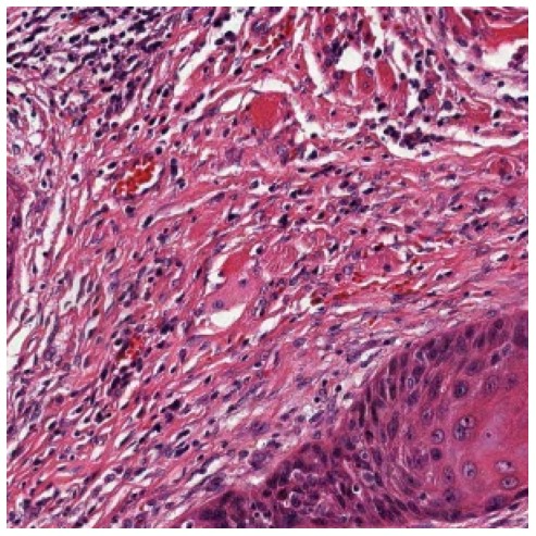
There are several ways you might acquire an image to use for a saliency map. To load an image tile from a whole-slide image, you can index a slideflow.WSI object:

import slideflow as sf

# Load a whole-slide image.
wsi = sf.WSI('slide.svs', tile_px=299, tile_um=302)

# Extract a tile using grid indexing.
image = wsi[10, 25]

Alternatively, if you know the coordinates for an image tile and want to extract it from TFRecords, you can use slideflow.Dataset.read_tfrecord_by_location():

import slideflow as sf

# Load a project and dataset.
P = sf.Project(...)
dataset = P.dataset(tile_px=299, tile_um=302)

# Get the tile from slide "12345" at location (2000, 2000)
slide, image = dataset.read_tfrecord_by_location(
    slide='12345',
    loc=(2000, 2000)
)

Once you have an image and a loaded SaliencyMap object, you can calculate a saliency map from the preprocessed image:

mask = sal_map.integrated_gradients(preprocess(image))

Plotting a Saliency Map¶

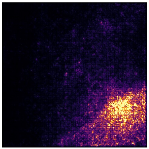
Once a saliency map has been created, you can plot the image as a heatmap or as an overlay. The slideflow.grad submodule includes several utility functions to assist with plotting. For example, to plot a basic heatmap using the inferno matplotlib colormap, use slideflow.grad.plot_utils.inferno():

from PIL import Image
from slideflow.grad.plot_utils import inferno

pil_image = Image.fromarray(inferno(mask))
pil_image.show()

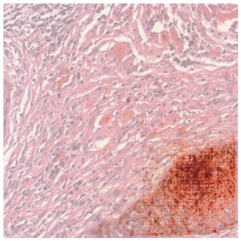
To plot this saliency map as an overlay, use slideflow.grad.plot_utils.overlay(), passing in both the unprocessed image and the saliency map:

from PIL import Image
from slideflow.grad.plot_utils import overlay

overlay_img = overlay(image.numpy(), mask)
pil_image = Image.fromarray(overlay_img)
pil_image.show()

Complete Example¶

The following is a complete example for how to calculate and plot a saliency map for an image tile taken from a whole-slide image.

import slideflow as sf
from slideflow.grad import SaliencyMap
from slideflow.grad.plot_utils import overlay
from PIL import Image

# Load a slide and find the desired image tile.
wsi = sf.WSI('slide.svs', tile_px=299, tile_um=302)
image = wsi[20, 20]

# Load a model and preprocessing function.
model = sf.model.load_model(../saved_model)
preprocess = sf.util.get_preprocess_fn('../saved_model')

# Prepare the saliency map
sal_map = SaliencyMap(model, class_idx=0)

# Calculate saliency map using integrated gradients.
ig_map = sal_map.integrated_gradients(preprocess(image))

# Display the saliency map as an overlay.
overlay_img = overlay(image, ig_map)
Image.fromarray(overlay_img).show()