Layer Activations
Investigating the latent space of a neural network can provide useful insights into the structure of your data and what models have learned during training. Slideflow provides several tools for post-hoc latent space analysis of trained neural networks, primarily by calculating activations at one or more neural network layers for all images in a dataset. In the next sections, we will take a look at how these layer activations can be calculated for downstream analysis and provide examples of analyses that can be performed.
Calculating Layer Activations
Activations at one or more layers of a trained network can be calculated with slideflow.model.Features and slideflow.DatasetFeatures. The former provides an interface for calculating layer activations for a batch of images, and the latter supervises calculations across an entire dataset.
Batch of images
Features provides an interface for calculating layer activations and predictions on a batch of images. The following arguments are available:
path: Path to model, from which layer activations are calculated. Required.layers: Layer(s) at which to calculate activations.include_preds: Also return the final network output (predictions)pooling: Apply pooling to layer activations, to reduce dimensionality to one dimension.
If layers is not supplied, activations at the post-convolutional layer will be calculated by default.
Once initialized, the resulting object can be called on a batch of images and will return the layer activations for all images in the batch. For example, to calculate activations at the sep_conv_3 layer of a model while looping through a dataset:
import slideflow as sf

sepconv3 = sf.model.Features('model/path', layer='sep_conv_3')
for img_batch in dataset:
    postconv_activations = sepconv3(img_batch)
If layer is a list of layer names, activations at each layer will be calculated and concatenated. If include_preds is True, the interface will also return the final predictions:
sepconv3_and_preds = sf.model.Features(..., include_preds=True)
layer_activations, preds = sepconv3_and_preds(img_batch)
Note
Features assumes that image batches already have any necessary preprocessing already applied, including standardization and stain normalization.
See the API documentation for Features for more information.
Single slide
Layer activations can also be calculated across an entire slide using the same Features interface. Calling the object on a slideflow.WSI object will generate a grid of activations of size (slide.grid.shape[0], slide.grid.shape[1], num_features):
import slideflow as sf

slide = sf.WSI(...)
postconv = sf.model.Features('/model/path', layers='postconv')
feature_grid = postconv(slide)
print(feature_grid.shape)
(50, 45, 2048)
Entire dataset
Finally, layer activations can also be calculated for an entire dataset using slideflow.DatasetFeatures. Instancing the class supervises the calculation and caching of layer activations, which can then be used for downstream analysis. The project function slideflow.Project.generate_features() creates and returns an instance of this class.
dts_ftrs = P.generate_features('/path/to/trained_model')
Alternatively, you can create an instance of this class directly:
import slideflow as sf

dataset = P.dataset(tile_px=299, tile_um=302)
dts_ftrs = sf.DatasetFeatures(
  model='/path/to/trained_model',
  dataset=dataset,
)
Tile-level feature activations for each slide can be accessed directly from DatasetFeatures.activations, a dict mapping slide names to numpy arrays of shape (num_tiles, num_features). Predictions are stored in DatasetFeatures.predictions, a dict mapping slide names to numpy arrays of shape (num_tiles, num_classes). Tile-level location data (coordinates from which the tiles were taken from their respective source slides) is stored in DatasetFeatures.locations, a dict mapping slide names to numpy arrays of shape (num_tiles, 2) (x, y).
Activations can be exported to a Pandas DataFrame with slideflow.DatasetFeatures.to_df() or exported into PyTorch format with slideflow.DatasetFeatures.to_torch(). See Generating Features for more information about generating and exporting features for MIL models.
Read the API documentation for slideflow.DatasetFeatures for more information.
Mapping Activations
Layer activations across a dataset can be dimensionality reduced with UMAP and plotted for visualization using slideflow.DatasetFeatures.map_activations(). This function returns an instance of slideflow.SlideMap, a class that provides easy access to labeling and plotting.
The below example calculates layer activations at the neural network layer sep_conv_3 for an entire dataset, and then reduces the activations into two dimensions for easy visualization using UMAP. Any valid UMAP parameters can be passed via keyword argument.
dts_ftrs = P.generate_features(
  model='/path/to/trained_model',
  layers='sep_conv_3'
)
slide_map = dts_ftrs.map_activations(
    n_neighbors=10, # UMAP parameter
    min_dist=0.2    # UMAP parameter
)
We can then plot the activations with slideflow.SlideMap.plot(). All keyword arguments are passed to the matplotlib scatter function.
import matplotlib.pyplot as plt

slide_map.plot(s=10)
plt.show()
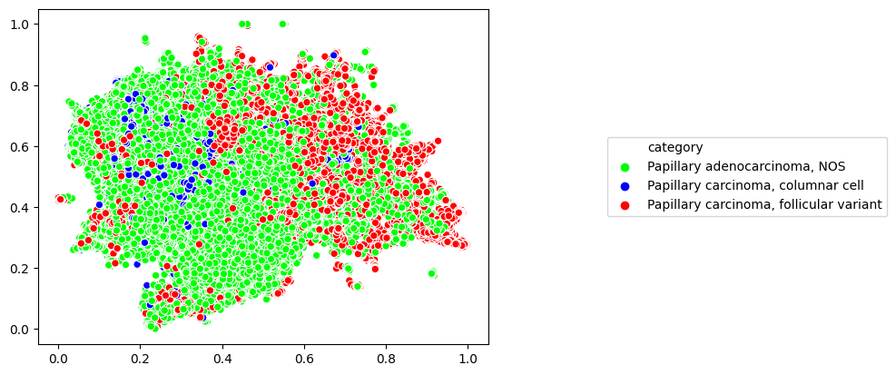
We can add labels to our plot by first passing a dictionary with slide labels to the function slideflow.SlideMap.label_by_slide().
# Get a dictionary mapping slide names to category labels
dataset = P.dataset(tile_px=299, tile_um='10x')
labels, unique_labels = dataset.labels('subtype', format='name')

# Assign the labels to the slide map, then plot
slide_map.label_by_slide(labels)
slide_map.plot()
Finally, we can use SlideMap.umap_transform() to project new data into two dimensions using the previously fit UMAP.
import slideflow as sf
import numpy as np

# Create a SlideMap using layer activations reduced with UMAP
dts_ftrs = P.generate_features(
  model='/path/to/trained_model',
  layers='sep_conv_3'
)
slide_map = dts_ftrs.map_activations()

# Load some dummy data.
# Second dimension must match size of activation vector.
dummy = np.random.random((100, 1024))

# Transform the data using the already-fit UMAP.
transformed = slide_map.umap_transform(dummy)
print(transformed.shape)
(100, 2)
Read more about additional slideflow.SlideMap functions, including saving, loading, and clustering, in the linked API documentation.
Mosaic Maps
Mosaic maps provide a tool for visualizing the distribution of histologic image features in a dataset through analysis of neural network layer activations. Similar to activation atlases, a mosaic map is generated by first calculating layer activations for a dataset, dimensionality reducing these activations with UMAP, and then overlaying corresponding images in a grid-wise fashion.
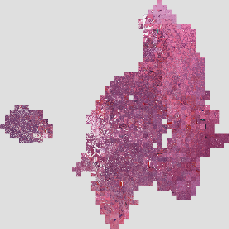
In the previous sections, we reviewed how to calculate layer activations across a dataset, and then dimensionality reduce these activations into two dimensions using UMAP. slideflow.Mosaic provides a tool for converting these activation maps into a grid of image tiles plotted according to their associated activation vectors.
Quickstart
The fastest way to build a mosaic map is using slideflow.Project.generate_mosaic, which requires a DatasetFeatures object as its only mandatory argument and returns an instance of slideflow.Mosaic.
dts_ftrs = P.generate_features('/path/to/trained_model', layers='postconv')
mosaic = P.generate_mosaic(dts_ftrs)
mosaic.save('mosaic.png')
When created with this interface, the underlying slideflow.SlideMap object used to create the mosaic map is accessible via slideflow.Mosaic.slide_map. You could, for example, use slideflow.SlideMap.save() to save the UMAP plot:
mosiac.slide_map.save('umap.png')
From a SlideMap
Any SlideMap can be converted to a mosaic map with slideflow.SlideMap.generate_mosaic().
ftrs = P.generate_features('/path/to/model')
slide_map = ftrs.map_activations()
mosaic = slide_map.generate_mosaic()
mosaic.save('mosaic.png')
Manual creation
Mosaic maps can be flexibly created with slideflow.Mosaic, requiring two components: a set of images and corresponding coordinates. Images and coordinates can either be manually provided, or the mosaic can dynamically read images from TFRecords (as is done with Project.generate_mosaic()).
The first argument of slideflow.Mosaic provides the images, and may be either of the following:
A list or array of images (np.ndarray, HxWxC)
A list of tuples, containing
(slide_name, tfrecord_index)
The second argument provides the coordinates:
A list or array of (x, y) coordinates for each image
For example, to create a mosaic map from a list of images and coordinates:
# Example data (images are HxWxC, np.ndarray)
images = [np.ndarray(...), ...]
coords = [(0.2, 0.9), ...]

# Generate the mosaic
mosaic = Mosaic(images, coordinates)
mosaic.plot()
You can also generate a mosaic map where the images are tuples of (tfrecord, tfrecord_index). In this case, the mosaic map will dynamically read images from TFRecords during plotting.
# Example data
tfrecords = ['/path/to/tfrecord`.tfrecords', ...]
idx = [253, 112, ...]
coords = [(0.2, 0.9), ...]

# Generate mosaic map
mosaic = sf.Mosaic(
    images=[(tfr, idx) for tfr, idx in zip(tfrecords, idx)],
    coords=coords
)
There are several additional arguments that can be used to customize the mosaic map plotting. Read the linked API documentation for slideflow.Mosaic for more information.