Tutorial 1: Model training (simple)

In this first tutorial, we will walk through the steps needed to take an example project from start to finish. As with all of these tutorials, we will use publicly available data from The Cancer Genome Atlas (TCGA). In this first tutorial, we will train a model to predict ER status from breast cancer slides.

Examples will be given assuming project files are in the directory /home/er_project and slides are in /home/brca_slides, although you will need to customize these paths according to your needs.

Create a Project

First, download slides and annotations for the TCGA-BRCA project using the legacy GDC portal. We should have a total of 1133 diagnostic slides across 1062 patients. Our outcome of interest is “er_status_by_ihc”, of which 1011 have a documented result (either “Positive” or “Negative”), giving us our final patient count of 1011.

Create a new project, and pass the path to the downloaded slides to the argument slides.

import slideflow as sf

P = sf.create_project(
    root='/home/er_project',
    slides='/path/to/slides'
)

After the project is created, we can load the project with:

P = sf.load_project('/home/er_project')

Setting up annotations

With our project initialized, we can set up our annotations file. Use the downloaded annotations file to create a new CSV file, with a column “patient” indicating patient name (in the case of TCGA, these are in the format TCGA-SS-XXXX, where SS indicates site of origin and XXXX is the patient identifier), and a column “er_status_by_ihc” containing our outcome of interest. Add a third column “slide” containing the name of the slide associated with the patient (without the file extension). If there are multiple slides per patient, list each slide on a separate row. Finally, add a column “dataset” to indicate whether the slide should be used for training or evaluation. Set aside somewhere around 10-30% of the dataset for evaluation.

Note

If patient names are identical to the slide filenames, the “slide” column does not need to be manually added, as slideflow will auto-associate slides to patients.

Your annotations file should look something like:

patient	er_status_by_ihc	dataset	slide
TCGA-EL-A23A	Positive	train	TCGA-EL-A3CO-01Z-00-DX1-7BF5F…
TCGA-EL-A24B	Negative	train	TCGA-EL-A24B-01Z-00-DX1-7BF5F…
TCGA-EL-A25C	Positive	train	TCGA-EL-A25C-01Z-00-DX1-7BF5F…
TCGA-EH-B31C	Negative	eval	TCGA-EH-B31C-01Z-00-DX1-7BF5F…
…	…	…	…

Save this CSV file in your project folder with the name annotations.csv.

Tile extraction

The next step is to extract tiles from our slides. For this example, we will use a 256px x 256px tile size, at 0.5 µm/pixel (128 um).

# Extract tiles at 256 pixels, 0.5 um/px
P.extract_tiles(tile_px=256, tile_um=128)

Hint

Tile extraction speed is greatly improved when slides are on an SSD or ramdisk; slides can be automatically buffered to an SSD or ramdisk directory by passing a directory to the argument buffer.

P.extract_tiles(256, 128, buffer='/mnt/ramdisk')

Training

After tiles are extracted, the dataset will be ready for training. We will train with a single set of manually defined hyperparameters, which we can configure with slideflow.ModelParams. We will use the Xception model with a batch size of 32, otherwise keeping defaults.

hp = sf.ModelParams(
    tile_px=256,
    tile_um=128,
    model='xception',
    batch_size=32,
    epochs=[3]
)

For training, we will use 5-fold cross-validation on the training dataset. To set up training, invoke the slideflow.Project.train() function with the outcome of interest, our hyperparameters, and our validation plan. We will use the filters argument to limit our training to the “train” dataset, as well as limit the training to only include patients with documented ER status (otherwise a blank “” would be marked as a third outcome).

# Train with 5-fold cross-validation
P.train(
    'er_status_by_ihc',
    params=hp,
    val_k_fold=5,
    filters={'dataset': ['train'],
                'er_status_by_ihc': ['Positive', 'Negative']}
)

After cross validation is complete, we will want to have a model trained across the entire dataset, so we can assess performance on our held-out evaluation set. To train a model across the entire training dataset without validation, we will set val_strategy to None:

# Train across the entire training dataset
P.train(
    'er_status_by_ihc',
    params=hp,
    val_strategy='none',
    filters={'dataset': ['train'],
                'er_status_by_ihc': ['Positive', 'Negative']}
)

Now, it’s time to start our pipeline. To review, our complete script should look like:

import slideflow as sf

# Create a new project
P = sf.create_project(
    root='/home/er_project',
    slides='/path/to/slides'
)

# Extract tiles at 256 pixels, 0.5 um/px
P.extract_tiles(tile_px=256, tile_um=128)

hp = ModelParams(
    tile_px=256,
    tile_um=128,
    model='xception',
    batch_size=32,
    epochs=[3, 5, 10]
)

# Train with 5-fold cross-validation
P.train(
    'er_status_by_ihc',
    params=hp,
    val_k_fold=5,
    filters={'dataset': ['train'],
                'er_status_by_ihc': ['Positive', 'Negative']}
)

# Train across the entire training dataset
P.train(
    'er_status_by_ihc',
    params=hp,
    val_strategy='none',
    filters={'dataset': ['train'],
                'er_status_by_ihc': ['Positive', 'Negative']}
)

The final training results should should show an average AUROC of around 0.87, with average AP around 0.83. Tile, slide, and patient-level receiver operator curves are saved in the model folder, along with precision-recall curves (not shown):

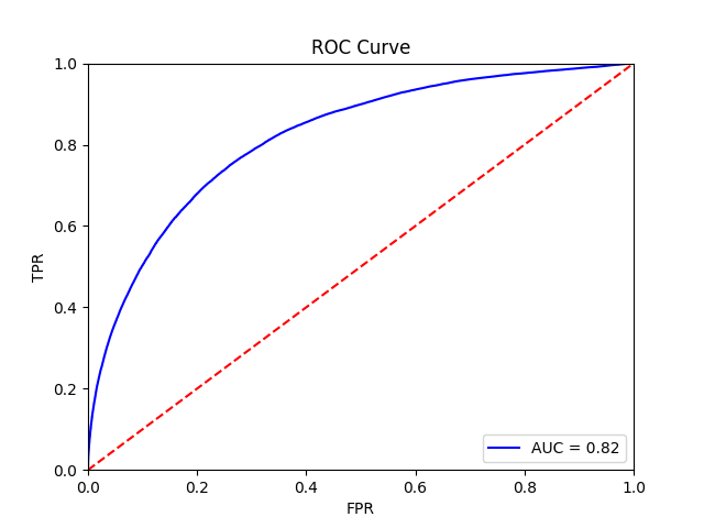
Tile-level receiver operator curve

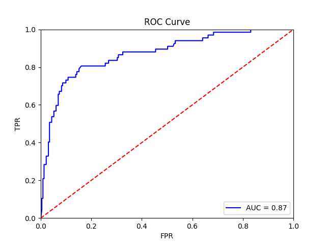
Patient-level receiver operator curve

Monitoring with Tensorboard

Tensorboard-formatted training and validation logs are saved the model directory. To monitor training with Tensorboard:

$ tensorboard --logdir=/project_path/models/00001-outcome-HP0

Tensorboard can then be accessed by navigating to https://localhost:6006 in a browser.