Multiple-Instance Learning (MIL)¶

In addition to standard tile-based neural networks, Slideflow also supports training multiple-instance learning (MIL) models. Several architectures are available, including attention-based MIL ("Attention_MIL"), CLAM ("CLAM_SB", "CLAM_MB", "MIL_fc", "MIL_fc_mc"), TransMIL ("TransMIL"), and HistoBistro Transformer ("bistro.transformer"). Custom architectures can also be trained. MIL training requires PyTorch.

Skip to Tutorial 8: Multiple-Instance Learning for a complete example of MIL training.

Generating features¶

The first step in MIL model development is generating features from image tiles. Many types of feature extractors can be used, including imagenet-pretrained models, models finetuned in Slideflow, histology-specific pretrained feature extractors (such as CTransPath or RetCCL), or fine-tuned SSL models. In all cases, feature extractors are built with slideflow.model.build_feature_extractor(), and features are generated for a dataset using either with slideflow.DatasetFeatures.to_torch() or slideflow.Project.generate_feature_bags().

Pretrained Feature Extractor¶

Slideflow includes several pathology-specific pretrained feature extractors:

Use slideflow.model.build_feature_extractor() to build one of these feature extractors by name. Weights for these pretrained networks will be automatically downloaded.

ctranspath = build_feature_extractor('ctranspath', tile_px=299)

ImageNet Features¶

To calculate features from an ImageNet-pretrained network, first build an imagenet feature extractor with slideflow.model.build_feature_extractor(). The first argument should be the name of an architecture followed by _imagenet, and the expected tile size should be passed to the keyword argument tile_px. You can optionally specify the layer from which to generate features with the layers argument; if not provided, it will default to calculating features from post-convolutional layer activations. For example, to build a ResNet50 feature extractor for images at 299 x 299 pixels:

from slideflow.model import build_feature_extractor

resnet50 = build_feature_extractor(
    'resnet50_imagenet',
    tile_px=299
)

This will calculate features using activations from the post-convolutional layer. You can also concatenate activations from multiple neural network layers and apply pooling for layers with 2D output shapes.

resnet50 = build_feature_extractor(
    'resnet50_imagenet',
    layers=['conv1_relu', 'conv3_block1_2_relu'],
    pooling='avg',
    tile_px=299
)

If a model architecture is available in both the Tensorflow and PyTorch backends, Slideflow will default to using the active backend. You can manually set the feature extractor backend using backend.

# Create a PyTorch feature extractor
extractor = build_feature_extractor(
    'resnet50_imagenet',
    layers=['layer2.0.conv1', 'layer3.1.conv2'],
    pooling='avg',
    tile_px=299,
    backend='torch'
)

You can view all available feature extractors with slideflow.model.list_extractors().

Features from Finetuned Model¶

You can also calculate features from any model trained in Slideflow. The first argument to build_feature_extractor() should be the path of the trained model. You can optionally specify the layer at which to calculate activations using the layers keyword argument. If not specified, activations are calculated at the post-convolutional layer.

# Calculate features from trained model.
features = build_feature_extractor(
    '/path/to/model',
    layers='sepconv3_bn'
)

Self-Supervised Learning¶

Finally, you can also generate features from a trained self-supervised learning model (either SimCLR or DinoV2).

For SimCLR models, use 'simclr' as the first argument to build_feature_extractor(), and pass the path to a saved model (or saved checkpoint file) via the keyword argument ckpt.

simclr = build_feature_extractor(
    'simclr',
    ckpt='/path/to/simclr.ckpt'
)

For DinoV2 models, use 'dinov2' as the first argument, and pass the model configuration YAML file to cfg and the teacher checkpoint weights to weights.

dinov2 = build_feature_extractor(
    'dinov2',
    weights='/path/to/teacher_checkpoint.pth',
    cfg='/path/to/config.yaml'
)

Exporting Features¶

Once you have prepared a feature extractor, features can be generated for a dataset and exported to disk for later use. Pass a feature extractor to the first argument of slideflow.Project.generate_feature_bags(), with a slideflow.Dataset as the second argument.

# Load a project and dataset.
P = sf.Project(...)
dataset = P.dataset(tile_px=299, tile_um=302)

# Create a feature extractor.
ctranspath = build_feature_extractor('ctranspath', tile_px=299)

# Calculate & export feature bags.
P.generate_feature_bags(ctranspath, dataset)

Note

If you are generating features from a SimCLR model trained with stain normalization, you should specify the stain normalizer using the normalizer argument to slideflow.Project.generate_feature_bags() or slideflow.DatasetFeatures.

Features are calculated for slides in batches, keeping memory usage low. By default, features are saved to disk in a directory named pt_files within the project directory, but you can override the destination directory using the outdir argument.

Alternatively, you can calculate features for a dataset using slideflow.DatasetFeatures and the .to_torch() method. This will calculate features for your entire dataset at once, which may require a large amount of memory. The first argument should be the feature extractor, and the second argument should be a slideflow.Dataset.

# Calculate features for the entire dataset.
features = sf.DatasetFeatures(ctranspath, dataset)

# Export feature bags.
features.to_torch('/path/to/bag_directory/')

Warning

Using slideflow.DatasetFeatures directly may result in a large amount of memory usage, particularly for sizable datasets. When generating feature bags for training MIL models, it is recommended to use slideflow.Project.generate_feature_bags() instead.

Feature “bags” are PyTorch tensors of features for all images in a slide, saved to disk as .pt files. These bags are used to train MIL models. Bags can be manually loaded and inspected using torch.load().

>>> import torch
>>> bag = torch.load('/path/to/bag.pt')
>>> bag.shape
torch.Size([2310, 768])
>>> bag.dtype
torch.float32

When image features are exported for a dataset, the feature extractor configuration is saved to bags_config.json in the same directory as the exported features. This configuration file can be used to rebuild the feature extractor. An example file is shown below.

{
 "extractor": {
  "class": "slideflow.model.extractors.ctranspath.CTransPathFeatures",
  "kwargs": {
   "center_crop": true
  }
 },
 "normalizer": {
  "method": "macenko",
  "fit": {
   "stain_matrix_target": [
    [
     0.5062568187713623,
     0.22186939418315887
    ],
    [
     0.7532230615615845,
     0.8652154803276062
    ],
    [
     0.4069173336029053,
     0.42241501808166504
    ]
   ],
   "target_concentrations": [
    1.7656903266906738,
    1.2797492742538452
   ]
  }
 },
 "num_features": 2048,
 "tile_px": 299,
 "tile_um": 302
}

The feature extractor can be manually rebuilt using slideflow.model.rebuild_extractor():

from slideflow.model import rebuild_extractor

# Recreate the feature extractor
# and stain normalizer, if applicable
extractor, normalizer = rebuild_extractor('/path/to/bags_config.json')

License & Citation¶

Licensing and citation information for the pretrained feature extractors is accessible with the .license and .citation attributes.

>>> ctranspath.license
'GNU General Public License v3.0'
>>> print(ctranspath.citation)

@{wang2022,
  title={Transformer-based Unsupervised Contrastive Learning for Histopathological Image Classification},
  author={Wang, Xiyue and Yang, Sen and Zhang, Jun and Wang, Minghui and Zhang, Jing  and Yang, Wei and Huang, Junzhou  and Han, Xiao},
  journal={Medical Image Analysis},
  year={2022},
  publisher={Elsevier}
}

Training¶

Model Configuration¶

To train an MIL model on exported features, first prepare an MIL configuration using slideflow.mil.mil_config().

The first argument to this function is the model architecture (which can be a name or a custom torch.nn.Module model), and the remaining arguments are used to configure the training process (including learning rate and epochs).

By default, training is executed using FastAI with 1cycle learning rate scheduling. Available models out-of-the-box include attention-based MIL ("Attention_MIL"), CLAM ("CLAM_SB", "CLAM_MB", "MIL_fc", "MIL_fc_mc"), transformer MIL ("TransMIL"), and HistoBistro Transformer ("bistro.transformer").

import slideflow as sf
from slideflow.mil import mil_config

config = mil_config('attention_mil', lr=1e-3)

Custom MIL models can also be trained with this API. Import a custom MIL model as a PyTorch module, and pass this as the first argument to slideflow.mil.mil_config().

import slideflow as sf
from slideflow.mil import mil_config
from my_module import CustomMIL

config = mil_config(CustomMIL, lr=1e-3)

Legacy CLAM Trainer¶

In addition to the FastAI trainer, CLAM models can be trained using the original CLAM training loop. This trainer has been modified, cleaned, and included as a submodule in Slideflow. This legacy trainer can be used for CLAM models by setting trainer='clam' for an MIL configuration:

config = mil_config(..., trainer='clam')

Training an MIL Model¶

Next, prepare a training and validation dataset and use slideflow.Project.train_mil() to start training. For example, to train a model using three-fold cross-validation to the outcome “HPV_status”:

...

# Prepare a project and dataset
P = sf.Project(...)
full_dataset = dataset = P.dataset(tile_px=299, tile_um=302)

# Split the dataset using three-fold, site-preserved cross-validation
splits = full_dataset.kfold_split(
    k=3,
    labels='HPV_status',
    preserved_site=True
)

# Train on each cross-fold
for train, val in splits:
    P.train_mil(
        config=config,
        outcomes='HPV_status',
        train_dataset=train,
        val_dataset=val,
        bags='/path/to/bag_directory'
    )

Model training statistics, including validation performance (AUROC, AP) and predictions on the validation dataset, will be saved in an mil subfolder within the main project directory.

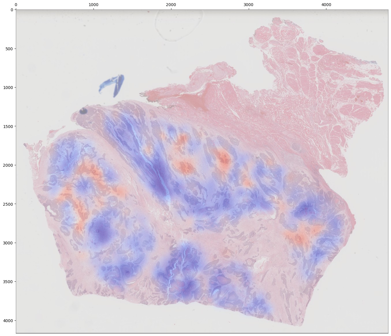
If you are training an attention-based MIL model (attention_mil, clam_sb, clam_mb), heatmaps of attention can be generated for each slide in the validation dataset by using the argument attention_heatmaps=True. You can customize these heatmaps with interpolation and cmap arguments to control the heatmap interpolation and colormap, respectively.

# Generate attention heatmaps,
# using the 'magma' colormap and no interpolation.
P.train_mil(
    attention_heatmaps=True,
    cmap='magma',
    interpolation=None
)

Hyperparameters, model configuration, and feature extractor information is logged to mil_params.json in the model directory. This file also contains information about the input and output shapes of the MIL network and outcome labels. An example file is shown below.

{
 "trainer": "fastai",
 "params": {

 },
 "outcomes": "histology",
 "outcome_labels": {
  "0": "Adenocarcinoma",
  "1": "Squamous"
 },
 "bags": "/mnt/data/projects/example_project/bags/simclr-263510/",
 "input_shape": 1024,
 "output_shape": 2,
 "bags_encoder": {
  "extractor": {
   "class": "slideflow.model.extractors.simclr.SimCLR_Features",
   "kwargs": {
    "center_crop": false,
    "ckpt": "/mnt/data/projects/example_project/simclr/00001-EXAMPLE/ckpt-263510.ckpt"
   }
  },
  "normalizer": null,
  "num_features": 1024,
  "tile_px": 299,
  "tile_um": 302
 }
}

Multi-Magnification MIL¶

Slideflow 2.2 introduced a multi-magnification, multi-modal MIL model, MultiModal_Attention_MIL ("mm_attention_mil"). This late-fusion multimodal model is based on standard attention-based MIL, but accepts multiple input modalities (e.g., multiple magnifications) simultaneously. Each input modality is processed by a separate encoder network and a separate attention module. The attention-weighted features from each modality are then concatenated and passed to a fully-connected layer.

Multimodal models are trained using the same API as standard MIL models. Modalities are specified using the bags argument to slideflow.Project.train_mil(), where the number of modes is determined by the number of bag directories provided. Within each bag directory, bags should be generated using the same feature extractor and at the same magnification, but feature extractors and magnifications can vary between bag directories.

For example, to train a multimodal model using two magnifications, you would pass two bag paths to the model. In this case, the /path/to/bags_10x directory contains bags generated from a 10x feature extractor, and the /path/to/bags_40x directory contains bags generated from a 40x feature extractor.

# Configure a multimodal MIL model.
config = mil_config('mm_attention_mil', lr=1e-4)

# Set the bags paths for each modality.
bags_10x = '/path/to/bags_10x'
bags_40x = '/path/to/bags_40x'

P.train_mil(
    config=config,
    outcomes='HPV_status',
    train_dataset=train,
    val_dataset=val,
    bags=[bags_10x, bags_40x]
)

You can use any number of modalities, and the feature extractors for each modality can be different. For example, you could train a multimodal model using features from a custom SimCLR model at 5x and features from a pretrained CTransPath model at 20x.

The feature extractors used for each modality, as specified in the bags_config.json files in the bag directories, will be logged in the final mil_params.json file. Multimodal MIL models can be interactively viewed in Slideflow Studio, allowing you to visualize the attention weights for each modality separately.

Evaluation¶

To evaluate a saved MIL model on an external dataset, first extract features from a dataset, then use slideflow.Project.evaluate_mil():

import slideflow as sf
from slideflow.model import build_feature_extractor

# Prepare a project and dataset
P = sf.Project(...)
dataset = P.dataset(tile_px=299, tile_um=302)

# Generate features using CTransPath
ctranspath = build_feature_extractor('ctranspath', tile_px=299)
features = sf.DatasetFeatures(ctranspath, dataset=dataset)
features.to_torch('/path/to/bag_directory')

# Evaluate a saved MIL model
P.evaluate_mil(
    '/path/to/saved_model'
    outcomes='HPV_status',
    dataset=dataset,
    bags='/path/to/bag_directory',
)

As with training, attention heatmaps can be generated for attention-based MIL models with the argument attention_heatmaps=True, and these can be customized using cmap and interpolation arguments.

Single-Slide Inference¶

Predictions can also be generated for individual slides, without requiring the user to manually generate feature bags. Use slideflow.model.predict_slide() to generate predictions for a single slide. The first argument is th path to the saved MIL model (a directory containing mil_params.json), and the second argument can either be a path to a slide or a loaded sf.WSI object.

from slideflow.mil import predict_slide
from slideflow.slide import qc

# Load a slide and apply Otsu thresholding
slide = '/path/to/slide.svs'
wsi = sf.WSI(slide, tile_px=299, tile_um=302)
wsi.qc(qc.Otsu())

# Calculate predictions and attention heatmap
model = '/path/to/mil_model'
y_pred, y_att = predict_slide(model, wsi)

The function will return a tuple of predictions and attention heatmaps. If the model is not attention-based, the attention heatmap will be None. To calculate attention for a model, set attention=True:

y_pred, y_att = predict_slide(model, slide, attention=True)

The returned attention values will be a masked numpy.ndarray with the same shape as the slide tile extraction grid. Unused tiles will have masked attention values.

Visualizing Attention Heatmaps¶

Attention heatmaps can be interactively visualized in Slideflow Studio by enabling the Multiple-Instance Learning extension (new in Slideflow 2.1.0). This extension is discussed in more detail in the Extensions section.